Linear Regression with one Variable in Matlab

In this post i will show you how to implement one of the basic Machine Learning concepts in Matlab, the Linear Regression with one Variable. Matlab and Octave are very useful high-level languages for prototyping Machine Learning algorithms.

 
[Linear Regression Example from mathworks.com]

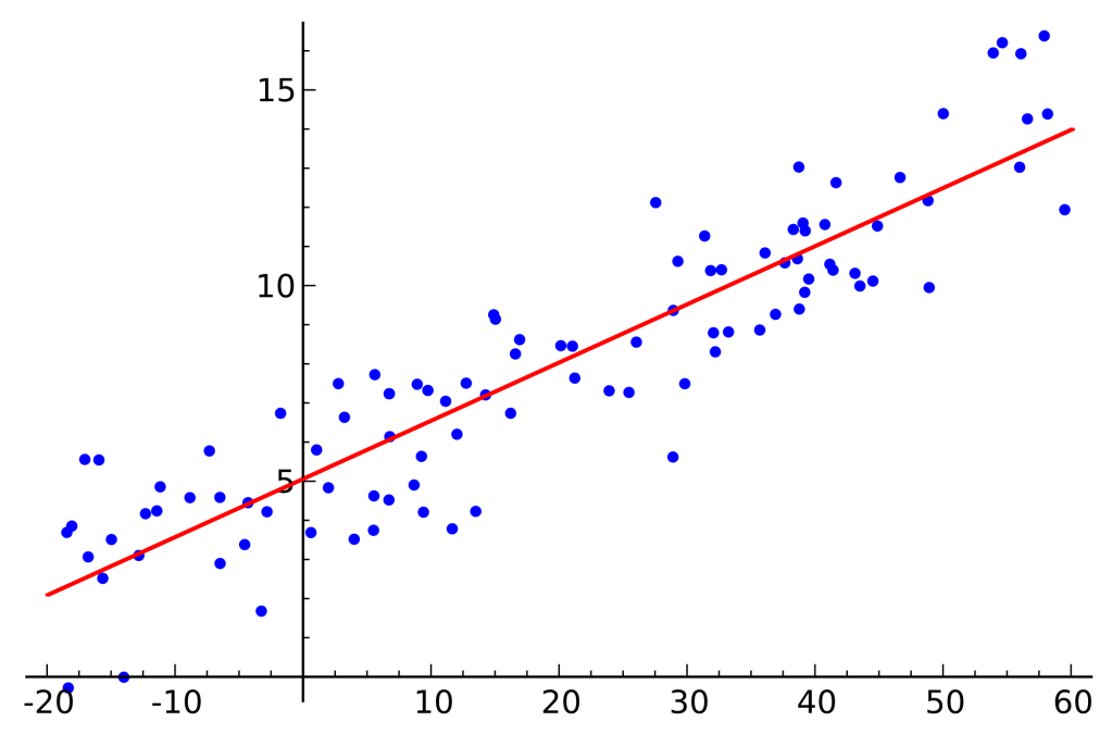
The idea is to find the line that perfectly fits all the dots in the diagram. This perfect fit line can be drawn using the fitting (Theta) parameters of the minimized function J for all data-points in the training data-set.

Lets assume that we have data with only one feature in txt format.

8.40840 7.22580
5.64070 0.71618
5.37940 3.51290
.
.
.
6.36540 5.30480
5.13010 0.56077
6.42960 3.65180
7.07080 5.38930

The first column X contains data-points which is our feature whose e.g. prices (second column y) we want to be able to predict using linear regression.

For the linear regression with one variable the minimized cost function consists of two fitting parameters Theta1 and Theta2 which are basically b and m in the line equation formula y=b+m*x.

The cost function has the following definition:

This cost-function can be implemented in two different ways. The first

% parameter m is the length of the training data-set.
squared_diff = 0;
%% v1
for i=1:m,
	x = X(i,:);,
 	squared_diff += (x*theta-y(i))^2;,
	%[x0,x1] = X(i,1);,
end

J = (1/(2*m))*squared_diff;

or more optimized way which uses build in functions of Matlab for calculating matrices and arrays:

%% v2
squared_error = sum(((X * theta) - y).^2);
J = (1/(2*m))*squared_error;

 

One of the possibilities to find the minimized cost function (minimal fitting parameters and ) is by using the Gradient Descent algorithm. The Gradient Descent algorithm uses the learning-rate (Alpha) parameter. This way the initial Theta parameters can be set to 0. The alpha parameter should be small to be able to converge at the end.

The Gradient Descent is defined as following:

In Matlab it can be implemented as following:

for iter = 1:num_iters
new_theta1 = theta(1) - alpha*(1/m)*sum(((X * theta) - y).*X(:,1));
new_theta2 = theta(2) - alpha*(1/m)*sum(((X * theta) - y).*X(:,2));

% sumultanious update
theta(1) = new_theta1;
theta(2) = new_theta2;

% Save the cost J in every iteration
cost = computeCost(X, y, theta);

end

 

If the parameters for alpha and num_iterations are carefully chosen the Gradient Descent should converge at the and and the regression line should have the perfect fit.

Cheers!