Have you ever asked yourself how the store managers decide on product shelf placement in retail stores? There must be some strategy behind it, right? It can’t be just a random choice. Almost on daily basis, you receive product purchase recommendations from variety of sources where you have left your “digital fingerprint”. In many cases these recommendations make sense, what leaves you puzzled, how did they figured it out?
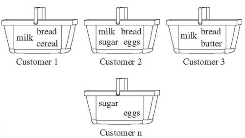
The Market Basket Analysis is perhaps the most famous method in Association Mining techniques arsenal. It’s all about finding frequent pairs, triples, quadruples of products from historical transactions or market baskets.
In this post I’ll show you small example how to implement Market Basket Analysis in Python. So let’s start…
btw… If you would like to go deeper into the topic of big data mining, find out more about this algorithm, and many others, check out this book! Mining of Massive Datasets. It is the single best source for big data mining and machine learning for massive datasets.

The picture below visualizes our historical transactions. For the sake of simplicity, there are only 8 transactions, from 0 to 7. Transaction number 2 implies the market basket containing Balsamico, Mozzarella and Wine. Basket number 5 contains only Pasta and Wine.

Each basket is a vector of bit values. Bit stands for 1 if the column product is in the basket, and 0 otherwise.
transaction_df = pd.DataFrame({'Beer' : [1,0,1,0,1,0,0,1],
                               'Coke' : [0,1,1,0,1,0,0,1],
                               'Pepsi' : [1,0,0,1,0,0,1,0],
                               'Milk' : [0,1,0,1,1,1,0,1],
                               'Juice' : [0,0,1,0,0,1,1,1]})
To ensure quality of the basket mining, it is important that every product, or at least most of them, is evenly distributed across all baskets. This feature of the transactional dataset is called product support. Let’s plot basket’s product support histogram.
# calculate occurrence(support) for every product in all transactions
product_support_dict = {}
for column in transaction_df.columns:
    product_support_dict[column] = sum(transaction_df[column]>0)

# visualise support
pd.Series(product_support_dict).plot(kind="bar")

We can see that every product in our transaction matrix is evenly distributed. That’s a good, and now we can start with frequent pairs mining.
Although this analysis can be implemented directly with pandas dataframe object, I choose to work with numpy matrices. I find that working with matrices is more natural than working with dataframes.
What the code below is doing, is basically taking every product’s vector and multiplying it with every other products vector. The final vector product of that multiplication indicates matches between products. Those matches indicate pairs. Summation of the matches gives us the pair frequency. The higher the number, the more frequent is the pair. The results are saved in new matrix (frequent_item_matrix).
# take data matrix from dataframe
transaction_matrix = transaction_df.as_matrix()
# get number of rows and columns
rows, columns = transaction_matrix.shape
# init new matrix
frequent_items_matrix = np.zeros((5,5))
# compare every product with every other
for this_column in range(0, columns-1):
    for next_column in range(this_column + 1, columns):
        # multiply product pair vectors
        product_vector = transaction_matrix[:,this_column] * transaction_matrix[:,next_column]
        # check the number of pair occurrences in baskets
        count_matches = sum((product_vector)>0)
        # save values to new matrix
        frequent_items_matrix[this_column,next_column] = count_matches

#print frequent_items_matrix
plot_matrix(frequent_items_matrix)
The resulting matrix looks like this:

Now, we only need to combine that resulting matrix with product names and we can get some meaningful information.
# and finally combine product names with data
frequent_items_df = pd.DataFrame(frequent_items_matrix, columns = transaction_df.columns.values, index = transaction_df.columns.values)

import seaborn as sns
# and plot
sns.heatmap(frequent_items_df)

And voila! We have our most frequent pairs. Who would have said that the Balsamico&Mozzarella and Balsamico&Pasta are the most frequent pairs 😉
Now, although we have the results, we could visualize the results differently or extract frequent pairs in another datastructure.
The code below extracts frequent pairs into new dictionary with pair as key and frequency as value.
# extract product pairs with minimum frequency(treshold) basket occurrences
def extract_pairs(treshold):
    output = {}
    # select indexes with larger or equal n
    matrix_coord_list = np.where(frequent_items_matrix >= treshold)
    # take values
    row_coords = matrix_coord_list[0]
    column_coords = matrix_coord_list[1]
    # generate pairs
    for index, value in enumerate(row_coords):
        #print index
        row = row_coords[index]
        column = column_coords[index]
        # get product names
        first_product = product_names[row]
        second_product = product_names[column]
        # number of basket matches
        matches = frequent_items_matrix[row,column]
        # put key values into dict
        output[first_product+"-"+second_product] = matches

    # return sorted dict
    sorted_output = OrderedDict(sorted(output.items(), key=lambda x: x[1]))
    return sorted_output

# plot pairs with minimum frequency of 1 basket matches
pd.Series(extract_pairs(1)).plot(kind="barh")

So there we have our pairs 🙂
Please note that this algorithm has execution time near O(n^2), or N over 2 pair combinations, and needs almost as much space, thus not suitable for mining frequent associations with large number of products. Check the Apriori algorithm for implementation with large data sets.
Here’s the full source.
This file contains hidden or bidirectional Unicode text that may be interpreted or compiled differently than what appears below. To review, open the file in an editor that reveals hidden Unicode characters.
Learn more about bidirectional Unicode characters
| # coding: utf-8 | |
| # In[41]: | |
| import numpy as np | |
| import scipy as sc | |
| from pandas import Series,DataFrame | |
| import pandas as pd | |
| import matplotlib.pyplot as plt | |
| import matplotlib as mpl | |
| import seaborn as sns | |
| from collections import OrderedDict | |
| from fractions import Fraction | |
| get_ipython().magic(u'matplotlib inline') | |
| mpl.rcParams['figure.figsize'] = (10.0, 5) | |
| # In[42]: | |
| # nice to have | |
| def plot_matrix(matrix): | |
| fig = plt.figure() | |
| ax = fig.add_subplot(111) | |
| cax = ax.matshow(matrix, interpolation='nearest') | |
| fig.colorbar(cax) | |
| # In[106]: | |
| transaction_df = pd.DataFrame({'Mozzarella' : [1,0,1,0,1,0,0,1], | |
| 'Balsamico' : [0,1,1,0,1,0,0,1], | |
| 'Pepsi' : [1,0,0,1,0,0,1,0], | |
| 'Pasta' : [0,1,0,1,1,1,0,1], | |
| 'Wine' : [0,0,1,0,0,1,1,1]}) | |
| transaction_df | |
| # In[107]: | |
| # calculate support for every product in all transactions | |
| product_support_dict = {} | |
| for column in transaction_df.columns: | |
| product_support_dict[column] = sum(transaction_df[column]>0) | |
| # visualise support | |
| pd.Series(product_support_dict).plot(kind="bar") | |
| # In[108]: | |
| transaction_matrix = transaction_df.as_matrix() | |
| transaction_matrix | |
| # In[109]: | |
| bool_index = (transaction_matrix>0) | |
| bool_index | |
| # In[110]: | |
| plot_matrix(transaction_matrix) | |
| # In[111]: | |
| # get number of rows and columns | |
| rows, columns = transaction_matrix.shape | |
| # init new matrix | |
| frequent_items_matrix = np.zeros((5,5)) | |
| # compare every product with every other | |
| for this_column in range(0, columns-1): | |
| print "this:", this_column,":",transaction_df.columns[this_column] | |
| for next_column in range(this_column + 1, columns): | |
| print "\tnext:", next_column,":",transaction_df.columns[next_column] | |
| # multiply product pair vectors | |
| product_vector = transaction_matrix[:,this_column] * transaction_matrix[:,next_column] | |
| # check the number of pair occurrences in baskets | |
| count_matches = sum((product_vector)>0) | |
| print "\t", count_matches | |
| # save values to new matrix | |
| frequent_items_matrix[this_column,next_column] = count_matches | |
| # In[112]: | |
| print frequent_items_matrix | |
| # In[113]: | |
| plot_matrix(frequent_items_matrix) | |
| # In[114]: | |
| # combine matrix with names | |
| frequent_items_df = pd.DataFrame(frequent_items_matrix, columns = transaction_df.columns.values, index = transaction_df.columns.values) | |
| sns.heatmap(frequent_items_df) | |
| # In[115]: | |
| product_names = transaction_df.columns.values | |
| # extract product pairs with minimum frequency(treshold) basket occurrences | |
| def extract_pairs(treshold): | |
| output = {} | |
| # select indexes with larger or equal n | |
| matrix_coord_list = np.where(frequent_items_matrix >= treshold) | |
| # take values | |
| row_coords = matrix_coord_list[0] | |
| column_coords = matrix_coord_list[1] | |
| # generate pairs | |
| for index, value in enumerate(row_coords): | |
| #print index | |
| row = row_coords[index] | |
| column = column_coords[index] | |
| # get product names | |
| first_product = product_names[row] | |
| second_product = product_names[column] | |
| # number of basket matches | |
| matches = frequent_items_matrix[row,column] | |
| # put key values into dict | |
| output[first_product+"-"+second_product] = matches | |
| # return sorted dict | |
| sorted_output = OrderedDict(sorted(output.items(), key=lambda x: x[1])) | |
| return sorted_output | |
| # plot pairs with minimum frequency of 2 basket matches | |
| min_frequency = 1 | |
| ax = pd.Series(extract_pairs(min_frequency)).plot(kind="barh", title="Frequent Pairs with Frequency >= " + str(min_frequency)) |
You can also find the source @https://github.com/dzenanh/mmds.
‘Nuff said. Enjoy the source. Cheers!

Leave a comment